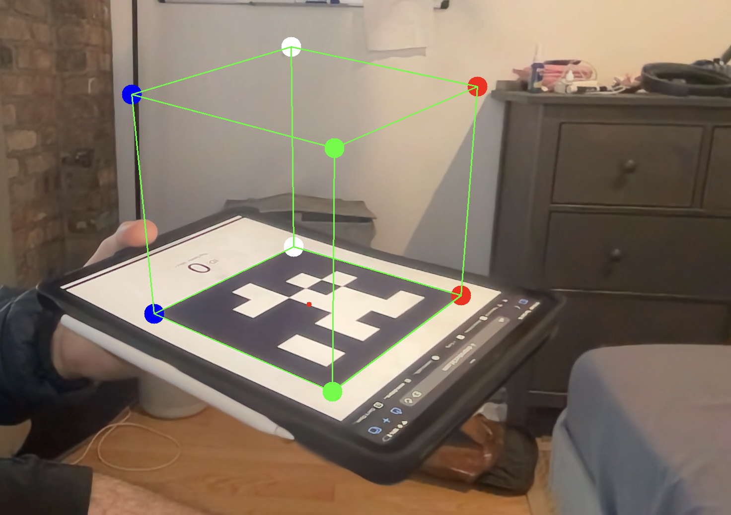
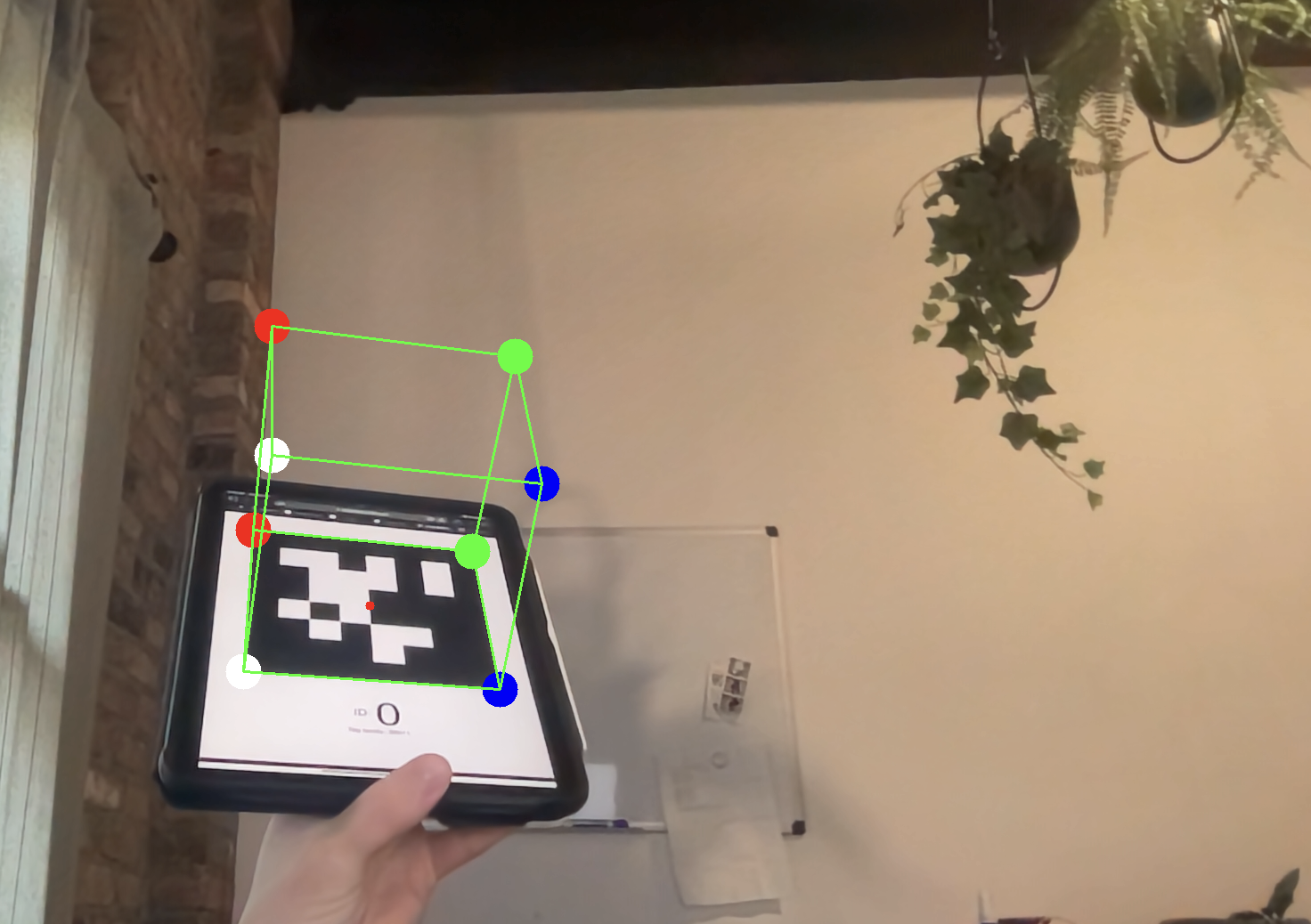
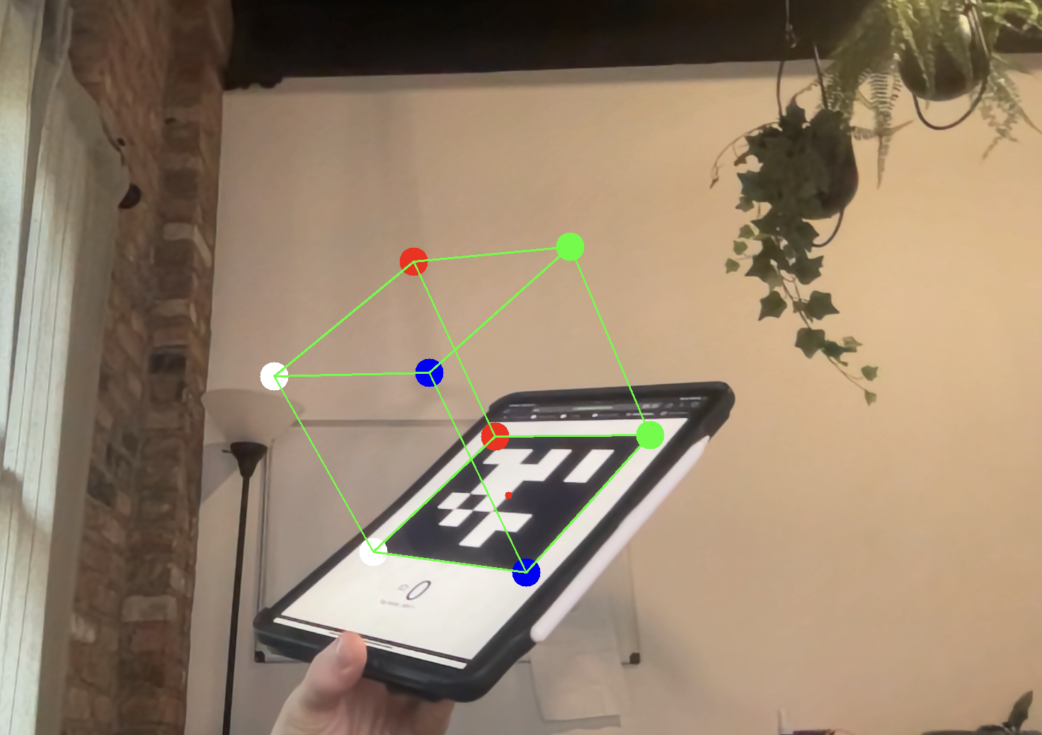
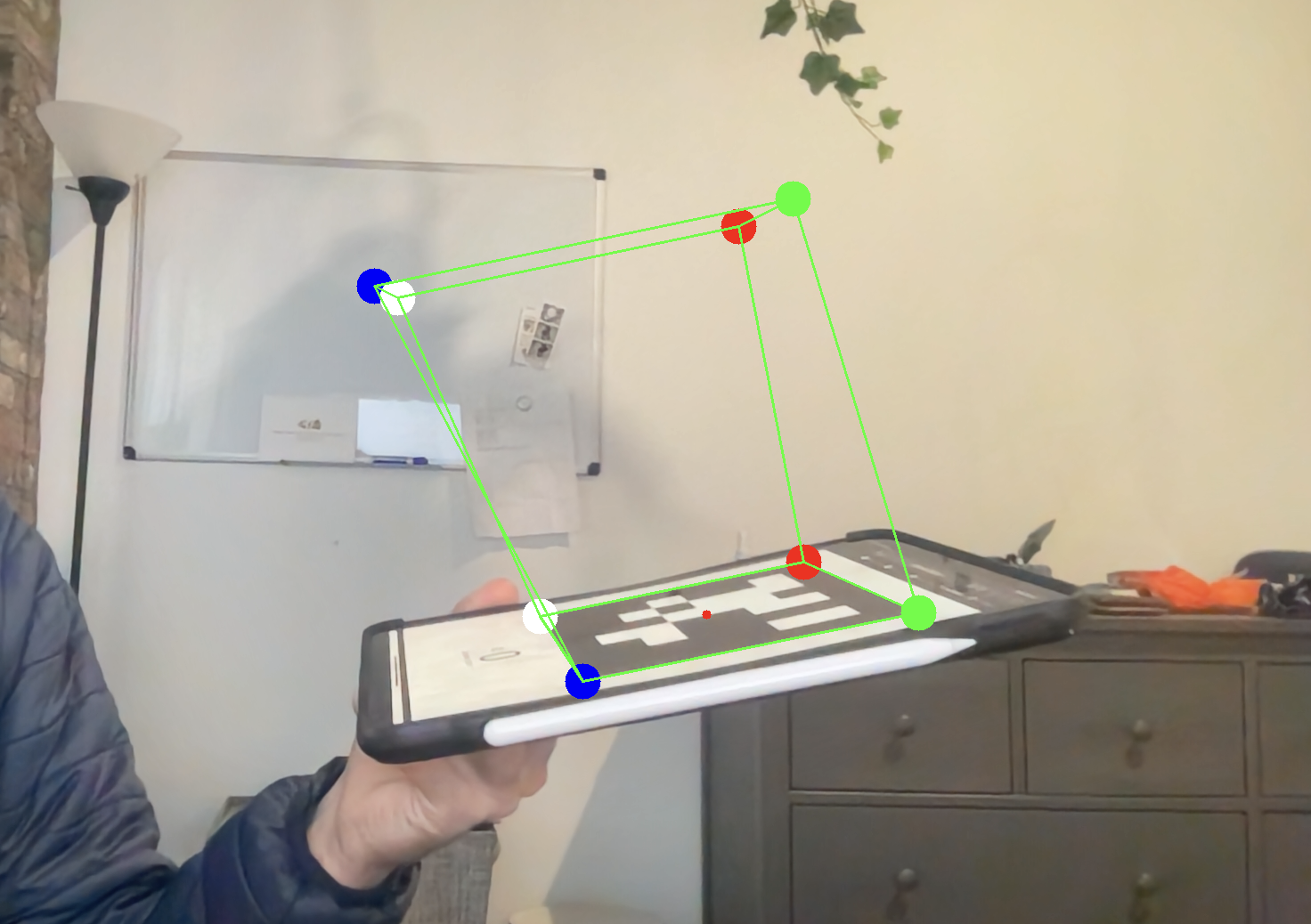
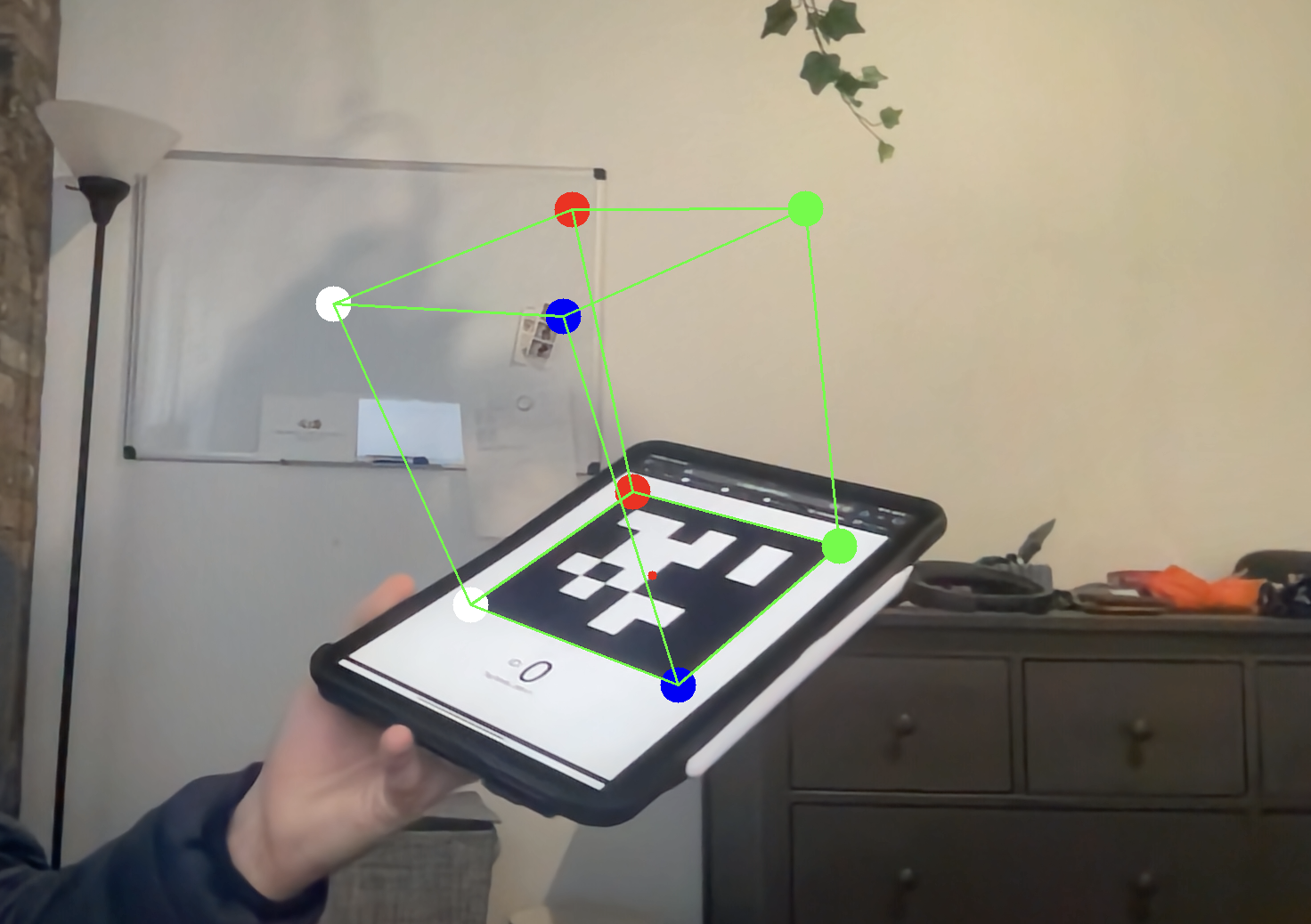
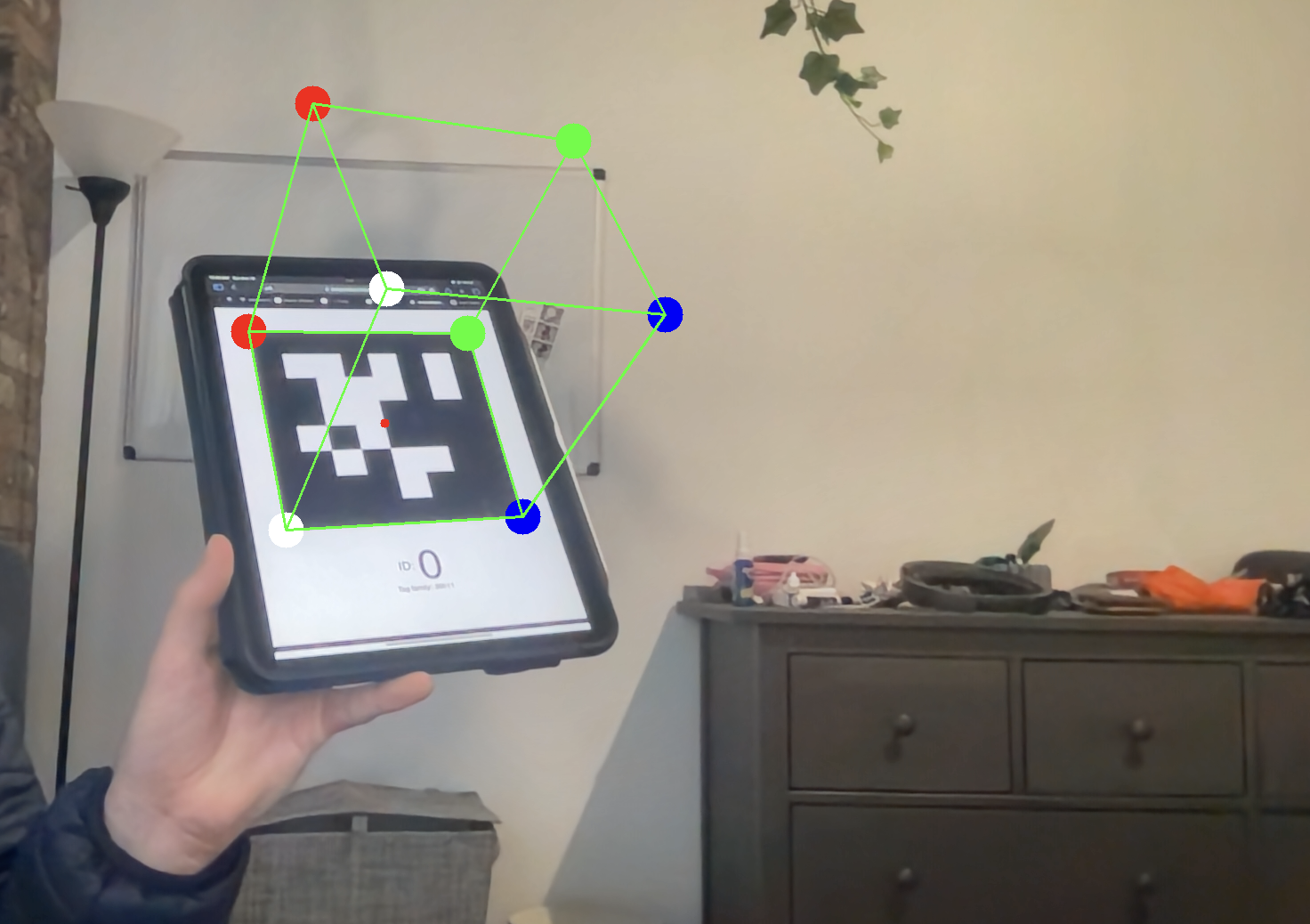
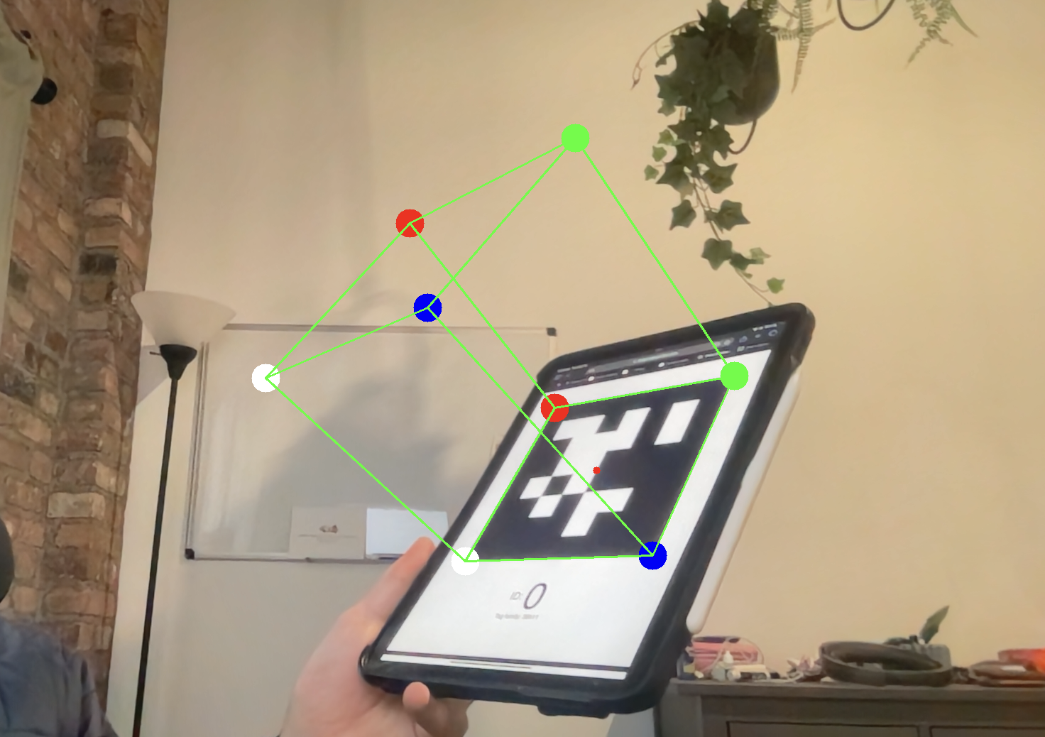
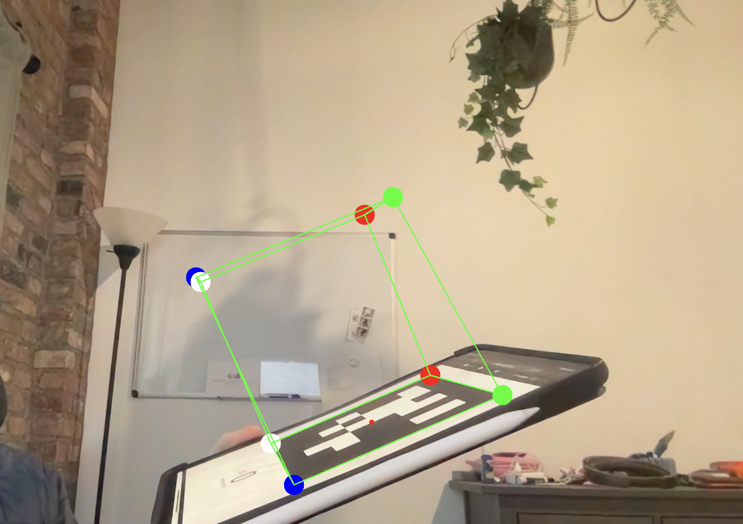
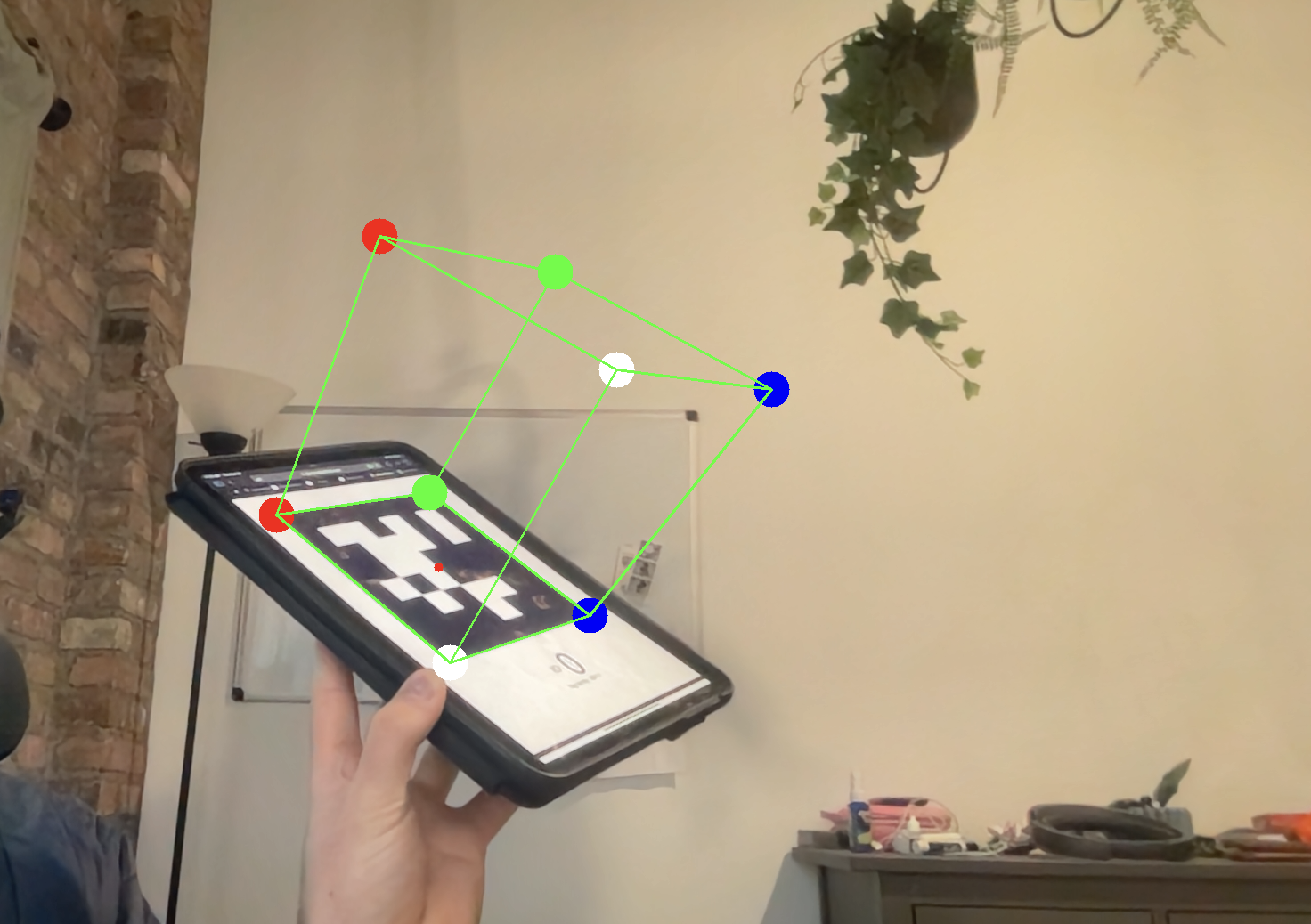
AR projection of Cube onto Fiducial marking

Overview

Hi, today we will be learning the basics of pose estimation using an image of a fiducial tag. This is extremely useful in all sorts of robotics and computer vision applications. We will be leveraging this technique to create an AR cube that will sit on the imaged marker.

This problem essentially boils down to three primary steps: estimating the homography of the AprilTag, extracting the orientation and position of the camera with relation to a frame attached to the AprilTag, then using that information to project points into the image plane as if you were imaging a box at the AprilTag frame.

What is a homography you ask? The pure mathematical definition is that it is a transformation that preserves collinearity. Practically however, it is a transformation that encodes the relative position of a known shape to the observer based on the way the known shape warps due to perspective geometry.

Imagine I show you a square, and you remember the observed size. I ask you to close your eyes, and I move the square to an distance farther away and at an angle. When you next see the square, based on the original information, you would be able to infer distance (due to change in scale) and angle (due to changes in perceived angles between sides of the square). This is exactly how we use a homography and a known square (the marker) to extract relative pose information.

I did this problem two ways: the easy way and the hard way. Both problems consisted initially of a detector that detected the AprilTags and returned the pixel locations of the AprilTag corners.

Operating

If you want to see the code itself, you can clone my repository and run the code. It should work as advertised.

Easy way

Using cv2.solvePnP, you can solve for the camera extrinsics by passing in the perceived AprilTags corners, the generally defined location of the AprilTag corners in the AprilTag frame (namely \([[0,0,0],[0,1,0],[1,1,0],[1,0,0]]\)), and the intrinsics of the camera. This function is very helpful for a couple reasons. The PnP problem is actually degenerate when you have four coplanar points (like in our case). However, the function automatically reverts to estimating the pose of the camera using homography estimation. It will return a angle-axis rotational parameterization of the orientation of the camera, along with a translation vector. These are exactly what we need to pass into our next function.

For this next section, its important to know the following equation:

\[s\begin{bmatrix} u\\v\\1 \end{bmatrix} = K \begin{bmatrix} R|t \end{bmatrix} \begin{bmatrix} X\\Y\\Z\\1 \end{bmatrix}\]

This is the so-called camera projection equation, and it essentially tells you, given the intrinsic and extrinsic parameters of the camera, how points in the real world are imaged in the image plane, up to a scale. This is important because, if we know where we want our cube to be in the world frame, the pose of the camera in the world frame, and our intrinsic camera parameters, we can compute the exact location of the cube as it would be imaged!

You can use projectPoints, which does this math for you, to compute the imaged locations of the imaginary cube’s corners. You can then draw lines connecting the corners. Its really that simple! As you rotate the tag, you should see the cube follow the motion of the tag.

Hard Way

The hard way is to essentially code all the steps yourself. The first two steps use my own implementation, and while I still use projectPoints, its really just a few easy matrix equations away from your own implementation.

You can find my implementation of the DLT algorithm that, with the corners in the global frame and image plane, constructs a \(Ax=0\) equation. I highly reccomend reading the Hartley-Zisserman Multiview Geometry book if you need proof why this makes sense. You can find it here. Using singular value decomposition, I can then exract the estimated homography from these points. In general, mo’ points means mo’ better, but since a homograhpy has 8 DOF, you need a minumum four points (i.e the four corners of the tag). To finish, I divide the entire matrix by a scalar of H[3,3] to ensure that the last element in the H matrix is 1.

For this next part, we want to remember the camera projection equation:

\[s\begin{bmatrix} u\\v\\1 \end{bmatrix} = K \begin{bmatrix} R|t \end{bmatrix} \begin{bmatrix} X\\Y\\Z\\1 \end{bmatrix}\]

To extract the rotation and translation from the homography, one uses a simple decomposition of the projection matrix P, defined here

\[p = K \begin{bmatrix} R|t \end{bmatrix}\]

We know that P is equal to H, as the definition of a homography is a 2D-2D planar transformation of points that preserves only collinearity. The projection equation follows this exact definition, as it projects the 2D points on the imaged tag to the image plane. Thus

\[H = K \begin{bmatrix} R|t \end{bmatrix}\]

By premultiplying the homography by \(K^{-1}\), I can extract the columns \(r_1\) and \(r_2\). This is confusing, but clear from the following equations:

\[K^{-1}H = \begin{bmatrix} R|t \end{bmatrix}\] \[K^{-1}H \begin{bmatrix} u\\v\end{bmatrix} = \begin{bmatrix} r_1 & r_2 & r_3 & t \end{bmatrix} \begin{bmatrix} X\\Y\\0 \end{bmatrix}\] \[\begin{bmatrix} K^{-1}H \end{bmatrix} = \begin{bmatrix} r_1 & r_2 & t \end{bmatrix}\]

Because the we define the world frame on the fiducial, the Z coordinate for our global frame points will always be zero. This allows us to eliminate the \(r_3\) vector and make the claim that \(r_1\), \(r_2\), and \(t\) are simply the column vectors of \(K^{-1}H\). We then normalize the column vectors of the H matrix by the average of the magnitudes \(\| r_1 \|\) and \(\|r_2\|\) to create vectors as close to unity as possible.

We can simply recover the lost \(r_3\) by crossing our normalized \(r_1\) and \(r_2\). In my implementation, I found that normalizing the three column vectors by the average of \(r_1\) and \(r_2\) of the resulting matrix from \(K^{-1}H\) resulted in a better rotation matrix.

I have also implemented a basic least-squared optimizer option using singular value decomposition. This optmization is not as good as the solvePnP version, and reduces some stability of estimated rotataion matrix, but does create better solutions in general. You can activate it as you see fit.

From my resulting R and T, I can convert my R into a angle-axis representation using cv2.Rodrigues and then pass all of that into my projectPoints, as before. I can then draw lines between my projected points.

Comparison of approaches

The primary disadvantage to the self-implementation approach has is that I do not do a great job with (if any) least-squared optimization on the resulting R from step 2 to find a true orthonormal rotation matrix. This means in general my results are slightly less than ideal, however still quite good.

Conclusion

Today we learned about Homographies, and how we can use them to extract the local position of images markers with respect to the camera. This approach is very powerful, despite us using it for a silly augmented reality project. Using a marker localization, you can develop a number of sophisticated programs that interact with the environment in interesting ways. If you want to see more, you can check out my research where I use this approach to aid an operator teleoperate a robot for object manipulation.